This tutorial will give you an idea of many aspects of LaTeX. Normal distribution or Gauss distribution is a huge topic where many types of mathematical symbols and expressions are used.
But before that, let’s look at some uses of LaTeX. Which will help to represent different equations of normal distribution.
\documentclass{article}
\usepackage{amssymb}
\begin{document}
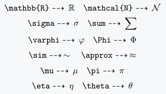
\[ \verb|\mathbb{R}| \dashrightarrow\,\mathbb{R}\quad\verb|\mathcal{N}|\dashrightarrow\,\mathcal{N} \]
\[ \verb|\sigma| \dashrightarrow\,\sigma\quad\verb|\sum|\dashrightarrow\,\sum \]
\[ \verb|\varphi| \dashrightarrow\,\varphi\quad\verb|\Phi|\dashrightarrow\,\Phi \]
\[ \verb|\sim|\dashrightarrow\,\sim \quad\verb|\approx|\dashrightarrow\,\approx \]
\[ \verb|\mu| \dashrightarrow\,\mu\quad\verb|\pi|\dashrightarrow\,\pi \]
\[ \verb|\eta| \dashrightarrow\,\eta\quad\verb|\theta|\dashrightarrow\,\theta \]
\end{document}Output :
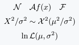
Also, know the use of one type of mathematical font. There is a default \mathcal{arg} command for this, which will return you a Calligraphic font style. However, this change is limited to the upper case letter.
\documentclass{article}
\begin{document}
  \[ \mathcal{N}\quad\mathcal{A}f(x)\quad\mathcal{F} \]
  \[ X^2/\sigma^2 \sim \mathcal{X}^2(\mu^2/\sigma^2) \]
  \[ \ln \mathcal{L}(\mu ,\sigma^2) \]
\end{document}
Output :
Normal distribution in LaTeX
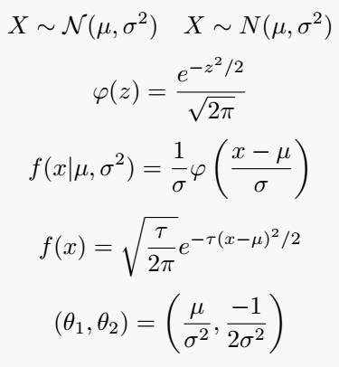
Below are some of your familiar equations or mathematical expressions with the help of LaTeX.
\documentclass{article}
\begin{document}
  \[ X\sim \mathcal{N}(\mu,\sigma^2)\quad X \sim N(\mu,\sigma^2) \]
  \[ \varphi(z)=\frac{e^{-z^2/2}}{\sqrt{2\pi}} \]
  \[ f(x|\mu ,\sigma^2)=\frac{1}{\sigma}\varphi\left(\frac{x-\mu}{\sigma}\right) \]
  \[ f(x)={\sqrt{\frac{\tau}{2\pi}}}e^{-\tau (x-\mu )^{2}/2} \]
  \[ (\theta_1 ,\theta_2)=\left(\frac{\mu}{\sigma^2},\frac{-1}{2\sigma^2}\right) \]
\end{document}
Output :
Calligraphic font style is also present in two more packages. Both calrsfs and euscript with the mathcal option packages have the same command.
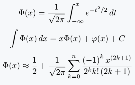
Common distribution function (cdf) in LaTeX
There are various equations for cdf whose source code is given below.
\documentclass{article}
\begin{document}
  \[ \Phi(x)={\frac{1}{\sqrt{2\pi}}}\int_{-\infty }^{x}e^{-t^{2}/2}\,dt \]
  \[ \int \Phi(x)\,dx=x\Phi (x)+\varphi(x)+C \]
  \[ \Phi(x)\approx {\frac{1}{2}}+{\frac {1}{\sqrt {2\pi }}}\sum_{k=0}^{n}{\frac {\left(-1\right)^{k}x^{\left(2k+1\right)}}{2^{k}k!\left(2k+1\right)}} \]
\end{document}
Output :
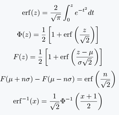
Cdf has an equation where the error function(erf) is denoted. However, you cannot write a latex function in direct math mode or text mode with normal fonts.
It is better to have predefined commands like \exp, \tan, \log etc. Otherwise you need to take the help of mathematical font. The \mathrm{arg} command below completes this task.
\documentclass{article}
\begin{document}
  \[ \mathrm{erf}(z)=\frac{2}{\sqrt{\pi}}\int_0^z e^{-t^2}dt \]
  \[ \Phi (z)={\frac{1}{2}}\left[1+\mathrm{erf}\left({\frac {z}{\sqrt{2}}}\right)\right] \]
  \[ F(z)=\frac{1}{2}\left[1+\mathrm{erf}\left(\frac{z-\mu}{\sigma{\sqrt{2}}}\right)\right] \]
  \[ F(\mu +n\sigma)-F(\mu -n\sigma)=\mathrm{erf}\left(\frac{n}{\sqrt{2}}\right) \]
  \[ \mathrm{erf}^{-1}(x)=\frac{1}{\sqrt{2}}\Phi^{-1}\left(\frac{x+1}{2}\right) \]
\end{document}
Output :