A column vector is a matrix whose elements are arranged sequentially along a column. Which you can easily represent with LaTeX.
Vertical continuous dots are used when the column vector carries n number of elements. Simple command for vertical dots is \vdots. What you need to know!
Let’s now define the matrix. start with the simple method, which is present in amsmath package.
I hope you know the syntax of Matrix, there is no problem if you don’t know, you will know.
\documentclass{article}
\usepackage{xcolor,amsmath}
\begin{document}
  \[
     \begin{pmatrix} v_1 \\ \vdots \\ v_n \end{pmatrix} \;
     \begin{bmatrix} w_1 \\ w_2 \\ \vdots \\ w_n \end{bmatrix} \;
     \begin{bmatrix} v_1w_1 \\ v_2w_2 \\ v_3w_3 \\ \vdots \\ v_nw_n \end{bmatrix}
  \]
  \[
     {\color{red}\vec{e}_x}=\begin{pmatrix} 1 \\ 0 \\ 0 \end{pmatrix},\;
     {\color{red}\vec{e}_y}=\begin{pmatrix} 0 \\ 1 \\ 0 \end{pmatrix},\;
     {\color{red}\vec{e}_z}=\begin{pmatrix} 0 \\ 0 \\ 1 \end{pmatrix}
  \]
\end{document}
Output :
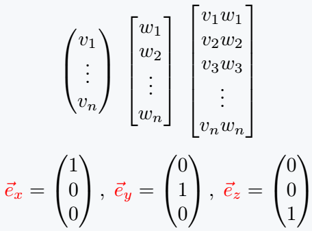
Notice in the code above, environment is used to define the matrix. And each vertical line is divided by \\.
Argument being passed to environment depends on what kind of brackets you want to enclose the matrix. For example, if you want brackets, you must pass bmatrix.
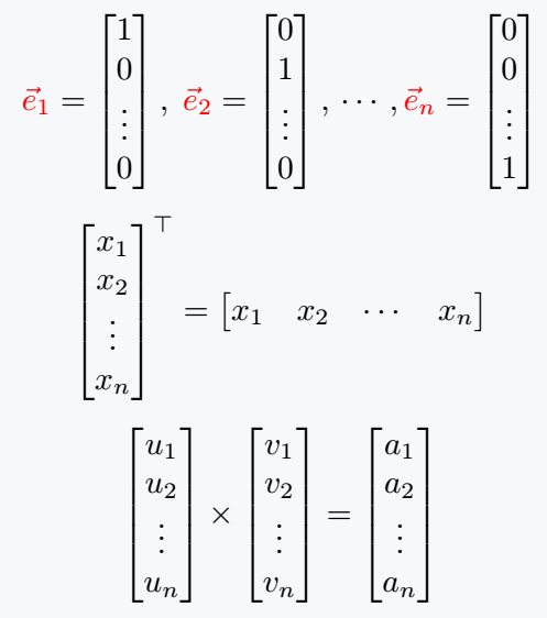
Below are some more mathematical expressions
\documentclass{article}
\usepackage{xcolor,amsmath}
\begin{document}
  \[
     {\color{red}\vec{e}_1}=\begin{bmatrix} 1 \\ 0 \\ \vdots \\ 0 \end{bmatrix},\;
     {\color{red}\vec{e}_2}=\begin{bmatrix} 0 \\ 1 \\ \vdots \\ 0 \end{bmatrix},\,\cdots,
     {\color{red}\vec{e}_n}=\begin{bmatrix} 0 \\ 0 \\ \vdots \\ 1\end{bmatrix}
  \]
  \[ \begin{bmatrix} x_1 \\ x_2 \\ \vdots \\ x_n \end{bmatrix}^\top = \begin{bmatrix} x_1 & x_2 & \cdots & x_n \end{bmatrix} \]
  \[ \begin{bmatrix} u_1 \\ u_2 \\ \vdots \\ u_n \end{bmatrix} \times \begin{bmatrix} v_1 \\ v_2 \\ \vdots \\ v_n \end{bmatrix} = \begin{bmatrix}  a_1 \\ a_2 \\ \vdots \\ a_n \end{bmatrix} \]
\end{document}
Output :
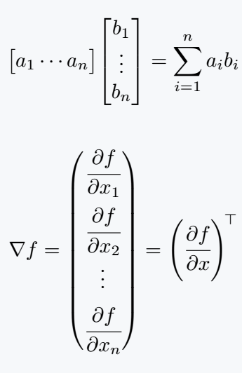
Use physics package for column vector
Environment is not required for physics package. Different commands are created for different matrices. Let’s look at the use of two of these commands, which are mqty and xmat.
Values must be passed into mqty commands in the same way that values were passed into the environment.
\documentclass{article}
\usepackage{physics}
\begin{document}
  \[ \mqty[a_1 \cdots a_n]\mqty[b_1 \\ \vdots \\b_n] = \sum _{i=1}^n a_ib_i \]
  \[ \nabla f =\mqty(\cfrac{\partial f}{\partial x_1} \vspace{.4em} \\ \cfrac{\partial f}{\partial x_2} \vspace{.1em} \\ \vdots \vspace{.4em} \\ \cfrac{\partial f}{\partial x_n}) = \left(\cfrac{\partial f}{\partial x}\right)^{\!\top} \]
\end{document}
Output :
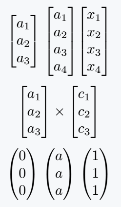
In the case of xmat command, elements of a matrix are filled with same constant number or variable. In this case, the structure of command is different which is given below
\xmat{variable/constant}{row number}{column number}
\documentclass{article}
\usepackage{physics}
\begin{document}
  \[ \mqty[\xmat*{a}{3}{1}] \; \mqty[\xmat*{a}{4}{1}] \mqty[\xmat*{x}{4}{1}] \]
  \[ \mqty[\xmat*{a}{3}{1}]\times \mqty[\xmat*{c}{3}{1}] \]
  \[ \mqty(\xmat{0}{3}{1}) \; \mqty(\xmat{a}{3}{1}) \; \mqty(\xmat{1}{3}{1}) \]
\end{document}
Output :
Jidan
LaTeX enthusiast and physics educator who enjoys explaining mathematical typesetting and scientific writing in a simple way. Writes tutorials to help students and beginners understand LaTeX more easily.