In LaTeX, curly brackets are essential, but they cannot be used directly like other brackets in a document.
\documentclass{article}
\begin{document}
   \[ {a_1,a_2, \cdots, a_n} \]
   \[ (b_1,b_2, \cdots, b_n) \]
   \[ [c_1,c_2, \cdots, c_n] \]
   \[ |d_1,d_2, \cdots, d_n| \]
\end{document}
Output :
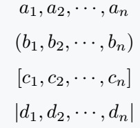
The solution is to place a backslash before each curly bracket. Let’s check if it works!
\documentclass{article}
\usepackage{amssymb}
\begin{document}
  \[ {a_1}, \{a_2\}, {a_3}, \{a_4\} \]
  \[ S_n = \{1,2,3,\cdots, n\} \]
  \[ S_n = \{a_1,a_2,a_3,\cdots, a_n\} \]
  % Don't used adjustable curly bracket
  \[ \mathbb{Q} = \{ \frac{p}{q} | a,b \in \mathbb{Z}, b\neq 0 \} \]
  \[ \{\frac{a_1}{n}\} , \{\frac{b_1}{m}\} , \{\frac{c_1}{k}\}\]
\end{document}
Output :
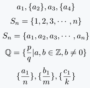
Table of Contents
Adjustable size of curly brackets
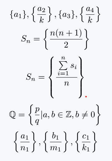
In the previous example, the mathematical expression was larger than the curly brackets, which might seem problematic.
However, LaTeX provides a simple solution with a built-in command that automatically adjusts bracket size to match the expression.
\documentclass{article}
\begin{document}
  \[ \{a_1\}, \left\{\frac{a_2}{k}\right\}, \{a_3\}, \left\{\frac{a_4}{k}\right\} \]
  \[ S_n = \left\{\frac{n(n+1)}{2}\right\} \]
  \[ S_n =\left\{\cfrac{\sum\limits_{i=1}^{n} {s_i}}{n}\right\} \]
  \[ \mathbb{Q} = \left\{ \frac{p}{q} | a,b \in \mathbb{Z}, b\neq 0 \right\} \]
  \[ \left\{\frac{a_1}{n_1}\right\} , \left\{\frac{b_1}{m_1}\right\} , \left\{\frac{c_1}{k_1}\right\} \]
\end{document}
Output :
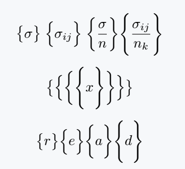
You can manually increase the bracket size, but this approach has limitations.
\documentclass{article}
\begin{document}
 \[ \big\{\sigma\big\} \; \Big\{\sigma_{ij}\Big\} \; \bigg\{\frac{\sigma}{n}\bigg\} \Bigg\{\frac{\sigma_{ij}}{n_k}\Bigg\} \]
 \[ \big\{ \Big\{ \bigg\{ \Bigg\{ x \Bigg\} \bigg\} \Big\} \big\} \]
 \[ \big\{ r \big\} \Big\{ e \Big\} \bigg\{ a \bigg\}  \Bigg\{ d\Bigg\} \]
\end{document}
Output :
Use newcommand
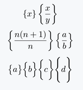
If you often use a specific curly bracket size, define a custom command with \newcommand for easy reuse throughout your document.
\documentclass{article}
\newcommand{\curly}[1]{\left\{ #1 \right\}}
\newcommand{\curlb}[2]{#1\{ #2 #1\}}
\begin{document}
 \[ \curly{x} \curly{\frac{x}{y}} \]
 \[ \curly{\frac{n(n+1)}{n}} \curly{\frac{a}{b}} \]
 \[ \curlb{\big}{a} \curlb{\Big}{b} \curlb{\bigg}{c} \curlb{\Bigg}{d} \]
\end{document}
Output :
Use physics package
The physics package includes a built-in command for curly brackets. Let’s explore its use!
\documentclass{article}
\usepackage{physics}
\begin{document}
 \[ \qty{x} \; \qty{\frac{x}{y}} \]
 \[ \qty{\frac{n^2 + 1}{n}} \]
 \[ \qty\big{m} \qty\Big{a} \qty\bigg{t} \qty\Bigg{h} \]
 \[\Bqty{\frac{n^2 + 2n + 1}{n}} \]
\end{document}
Output :
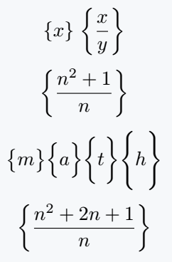
For \qty command, curly brackets will be automatically adjustable with expressions.
Along with \qty command, you can use the big command. But, in this case the process of using big command is completely different.
Use curly bracket in Matrix
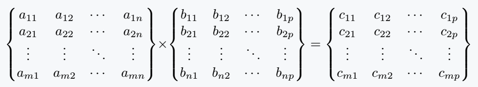
Matrices are enclosed in curly brackets by default. Simply pass the Bmatrix argument to the matrix environment no need for separate brackets.
\documentclass{article}
\usepackage{amsmath}
\begin{document}
 \[ \begin{Bmatrix}
         a_{11} & a_{12} & \cdots & a_{1n}\\
         a_{21} & a_{22} & \cdots & a_{2n}\\
         \vdots & \vdots & \ddots & \vdots\\
         a_{m1} & a_{m2} & \cdots & a_{mn}
     \end{Bmatrix}
     \times
     \begin{Bmatrix}
         b_{11} & b_{12} & \cdots & b_{1p}\\
         b_{21} & b_{22} & \cdots & b_{2p}\\
         \vdots & \vdots & \ddots & \vdots\\
         b_{n1} & b_{n2} & \cdots & b_{np}
     \end{Bmatrix}
      =
     \begin{Bmatrix}
         c_{11} & c_{12} & \cdots & c_{1p}\\
         c_{21} & c_{22} & \cdots & c_{2p}\\
         \vdots & \vdots & \ddots & \vdots\\
         c_{m1} & c_{m2} & \cdots & c_{mp}
     \end{Bmatrix} \]
\end{document}
Output :
Jidan
LaTeX enthusiast and physics educator who enjoys explaining mathematical typesetting and scientific writing in a simple way. Writes tutorials to help students and beginners understand LaTeX more easily.