Integration is a core part of mathematics, especially in calculus and scientific writing.
In LaTeX, different commands and packages help you write integrals clearly, whether it is a single integral, double or triple, or even a closed contour integral.
This guide shows all the main methods with examples.
Table of Contents
Basic Integral Symbol
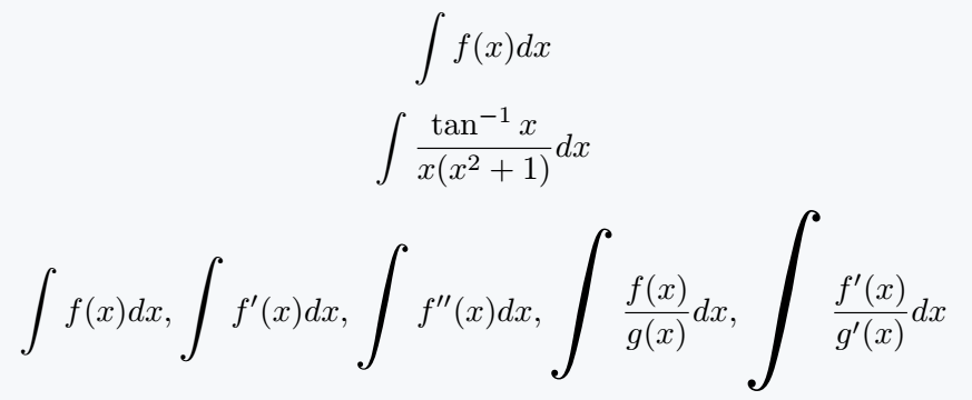
The default way to write an integral is with the \int command. By itself, it creates a normal-sized symbol.
If you need larger integral symbols, the bigints package lets you scale them step by step.
\int f(x) dx
\int- This produces the basic integral symbol used in most cases. It works in both inline and display mode.
f(x) dx- This is the integrand and the differential part. You can replace
f(x)with any function.
\documentclass{article}
\usepackage{bigints}
\begin{document}
   \[ \int f(x) dx \]
   \[ \int \frac{\tan^{-1}x}{x(x^2+1)}dx \]
   \[ \bigintssss f(x)dx ,\bigintsss f'(x)dx ,\bigintss f''(x)dx,\bigints \frac{f(x)}{g(x)}dx,\bigint \frac{f'(x)}{g'(x)}dx \]
\end{document}
Add Limits Above and Below
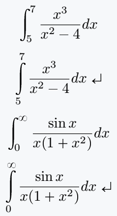
To show integration limits, you can add subscripts and superscripts. By default they appear on the side, but using \limits places them directly above and below the symbol.
\int_a^b f(x) dx
\int\limits_5^7 f(x) dx
_5^7- This sets the lower limit (a) and the upper limit (b) for the integral.
\limits- This forces the limits to appear above and below the integral symbol, instead of on the side.
\documentclass{article}
\begin{document}
   \[ \int_5^7 \frac{x^3}{x^2-4}dx \]
   \[ \int\limits_5^7 \frac{x^3}{x^2-4}dx \]
   \[ \int_0^\infty \frac{\sin x}{x(1+x^2)}dx \]
   \[ \int\limits_0^\infty \frac{\sin x}{x(1+x^2)}dx \]
\end{document}
Fixing Spacing Issues before {dx}
When writing integrals in LaTeX, you may notice that terms like xdx appear too close to each other.
To make your equations more readable, LaTeX provides spacing commands that let you add small amounts of space where needed.
\int x\,dx
\int x\:dx
\int x\;dx
\,- Thin space. Very small gap, often used between a variable and
dxin integrals. \:- Medium space. Slightly larger than
\,. \;- Thick space. Creates a noticeable gap between elements.
\documentclass{article}
\begin{document}
\[ \int_0^\infty \frac{\tan^{-1}x}{x^2+1}dx \]
\[ \int x{dx} \int x\,{dx} \int x\:{dx} \int x\;{dx} \]
\[ \int\limits_0^\infty \frac{\sin x}{x(x^2+1)}\;dx \]
\end{document}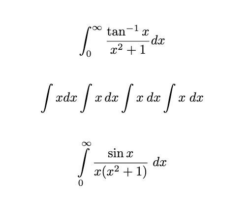
Custom Command with newcommand
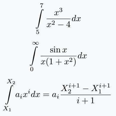
To avoid writing \limits and bounds every time, you can define a custom command. This makes integrals with limits faster and cleaner to write.
\newcommand{\integral}[2]{\int\limits_{#1}^{#2}}
\newcommand- Defines a new custom command in LaTeX.
{\intg}[2]- Here
\intgis the new command name and#1,#2are the lower and upper limits. \int\limits_{#1}^{#2}- This ensures that whenever you call
\integral, it produces a symbol with limits above and below.
\documentclass{article}
\usepackage{bigints}
\newcommand{\integral}[2]{\int\limits_{#1}^{#2}}
\begin{document}
   \[ \intg{5}{7} \frac{x^3}{x^2-4}dx \]
   \[ \intg{0}{\infty}\frac{\sin x}{x(1+x^2)}dx \]
   \[ \intg{X_1}{X_2}a_i x^i dx= a_i \frac{X^{i+1}_2 - X^{i+1}_1}{i+1}\]
\end{document}
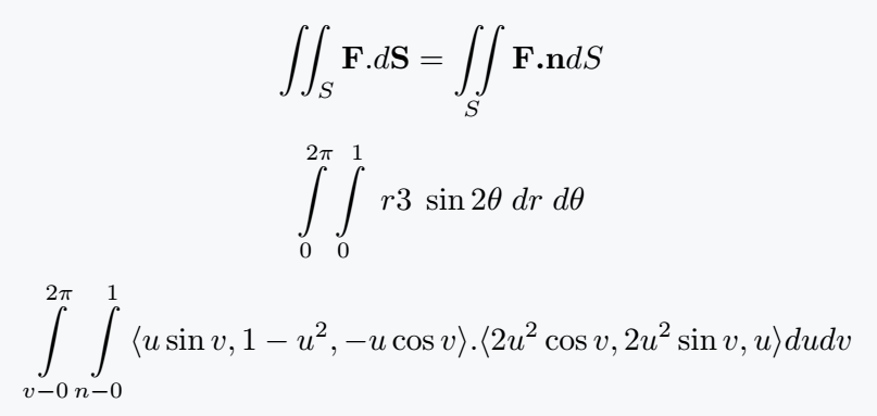
Double Integrals
For surface integrals or two-dimensional integration, you can use \iint. Each integral symbol can take its own set of limits.
You can also define them with \newcommand for consistency.
\documentclass{article}
\usepackage{amsmath}
\newcommand{\integral}[2]{\int\limits^{#1}_{#2}}
\begin{document}
   \[ \iint_S \textbf{F}.d\textbf{S}= \iint\limits_S \textbf{F.n}dS \]
   \[ \integral{2\pi}{0}\integral{1}{0} \;r3\; \sin 2\theta\; dr \;d\theta \]
   \[ \integral{2\pi}{v-0}\integral{1}{n-0}\langle u\sin v,1-u^2,-u\cos v\rangle.\langle 2u^2\cos v,2u^2 \sin v,u\rangle dudv \]
\end{document}
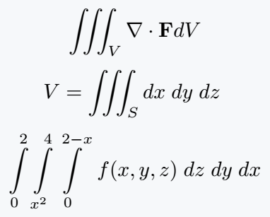
Triple Integrals
For volume integrals in three dimensions, LaTeX provides the \iiint command. It works like \iint but shows three integral symbols together.
\documentclass{article}
\usepackage{amsmath}
\newcommand{\integral}[2]{\int\limits^{#1}_{#2}}
\begin{document}
  \[ \iiint_V \nabla \cdot\textbf{F}dV \]
  \[ V =\iiint_S dx\; dy\; dz\; \]
  \[ \integral{2}{0}\integral{4}{x^2}\integral{2-x}{0}\; f(x,y,z)\;dz\;dy\;dx \]
\end{document}
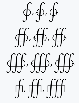
Closed Integrals
Closed path or contour integrals are written with the \oint family of commands. Packages like pxfonts, stix, and mathabx provide variants with clockwise, counterclockwise, and multiple integrals.
\documentclass{article}
\usepackage{pxfonts}
\begin{document}
  \[ \oint,\ointclockwise,\ointctrclockwise \]
  \[ \oiint,\oiintclockwise,\oiintctrclockwise  \]
  \[ \oiiint,\oiiintclockwise,\oiiintctrclockwise \]
  \[ \sqint,\sqiint,\sqiiint \]
\end{document}
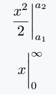
Evaluation Bar with Limits
To show the evaluation of an integral at bounds, you can either write it manually or use the \eval command from the physics package. It gives a clean notation for definite integrals.
\frac{x^2}{2} \bigg|_{a_1}^{a_2}
\eval{x}_0^\infty
\bigg|_{a_1}^{a_2}- The vertical bar with lower and upper values shows evaluation between
a₁anda₂. \eval- This command from the physics package automatically creates an evaluation bar.
{x}_0^\infty- The expression
xis evaluated from the lower limit0to the upper limit∞.
\documentclass{article}
\usepackage{physics}
\begin{document}
  \[\frac{x^2}{2} \bigg|_{a_1}^{a_2} \]
  \[ \eval{x}_0^\infty \]
\end{document}
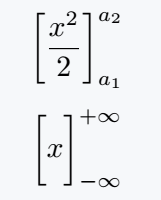
Square Brackets with Limits
Sometimes integrals are expressed with square brackets instead of a vertical bar. To ensure brackets scale properly, use \bigg or the \bqty command from the physics package.
\bigg[\frac{x^2}{2} \bigg]_{a_1}^{a_2}
\bigg[ ... \bigg]- The
\biggmakes the square brackets scale to fit the size of the content inside. _{a_1}^{a_2}- This places the lower and upper evaluation limits for the result of the integral.
\documentclass{article}
\usepackage{physics}
\begin{document}
  \[ \bigg[\frac{x^2}{2} \bigg]_{a_1}^{a_2} \]
  \[ \bqty\bigg{x}_{-\infty}^{+\infty} \]
\end{document}
Best Practice
For normal integrals, \int is enough, but use \limits when you want clear positioning of bounds. The bigints package is helpful if you need larger symbols in detailed documents.
For double and triple, prefer \iint and \iiint from amsmath. When dealing with closed paths, use packages like pxfonts or stix for contour integrals.
For evaluation, \eval from physics makes your work much cleaner. Choosing the right method depends on whether you need clarity for readers or compactness for inline math.
Jidan
LaTeX enthusiast and physics educator who enjoys explaining mathematical typesetting and scientific writing in a simple way. Writes tutorials to help students and beginners understand LaTeX more easily.