How to Write Partial Derivative(∂x/∂t) in LaTeX?

Partial derivatives are fundamental in calculus, physics, and engineering for representing how a function changes with respect to one variable while keeping others constant.

This guide explains how to typeset partial derivatives in LaTeX, from basic symbols to advanced macros in a structured and easy-to-follow way.

Basic Command

The simplest way to display a partial derivative symbol in LaTeX is by using the \partial command. This produces the symbol ∂, which is the standard notation for partial derivatives.

It is ideal when writing mathematical formulas directly, without additional packages.

\frac{\partial{f}}{\partial{x}}

• \frac

  This is the LaTeX command for a fraction. It creates a numerator and a denominator separated by a horizontal bar.

• \partial{f}

  This represents the partial derivative operator applied to a function f. It is used to show the differentiation of f with respect to one variable.

• \partial{x}

  This part of the fraction denotes the variable with respect to which the function is differentiated.

\documentclass{article}
\begin{document}
  By definition, let $u=u(x,y,z,t)$. The partial derivative of $u$ with respect to $x$ is 
  \[
     \frac{\partial u}{\partial x} = \lim_{\ell \to 0}\frac{u(x+\ell,y,z,t)-u(x,y,z,t)}{\ell}.
  \]
\end{document}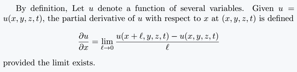

Below are the different notations for presenting the partial derivative of a function f with respect to x.

Notation	Command
	f’_{x}
	\partial_{x}f
	D_{x}f
	D_{1}f
	\frac{\partial}{\partial{x}}f
	\frac{\partial{f}}{\partial{x}}

Using Physics Package

The physics package simplifies writing partial derivatives through the \pdv command.

It automatically arranges the notation neatly, supports higher orders, and even mixed derivatives.

\pdv[n]{f}{x} \quad \pdv{f}{x}{y}

• \pdv

  This command from the physics package typesets partial derivatives. It automatically places \partial symbols and fractions correctly.

• [n]

  This optional argument denotes the order of the derivative, e.g., [2] for second order.

• {f}

  This argument is the function or expression to be differentiated.

• {x}

  This specifies the variable with respect to which differentiation is done.

\documentclass{article}
\usepackage{physics}
\begin{document}
  \[
    \pdv{f}{x}, \quad \pdv[2]{f}{x}, \quad \pdv{f}{x}{y}, \quad \pdv[n]{f}{x}.
  \]
\end{document}

Using Custom Macros

You can use \newcommand to define your own shorthand macros for partial derivatives. This helps avoid repetitive typing and keeps your code cleaner.

\newcommand{\pd}[2]{\frac{\partial #1}{\partial #2}}

• \newcommand

  Used to define a custom LaTeX command. It can take optional arguments for flexibility.

• {\pd}

  The custom name of the command, which can be used later in the document.

• {#1}, {#2}

  Placeholders for arguments passed to the command, where #1 is the numerator and #2 is the denominator.

\documentclass{article}
\newcommand{\pd}[2]{\frac{\partial #1}{\partial #2}}
\begin{document}
  \[
    \pd{u}{x}, \quad \pd{f}{y}.
  \]
\end{document}

Higher Order and Mixed Derivatives

You can typeset higher order derivatives by adjusting powers or stacking multiple \partial operators. For mixed derivatives, clearly show the order of differentiation.

\frac{\partial^2 f}{\partial x \partial y}

• \partial^2 f

  Represents the second-order partial derivative of f.

• \partial x \partial y

  Indicates that f is first differentiated with respect to y, then with respect to x.

\documentclass{article}
\begin{document}
  Mixed and higher order examples
  \[
    \frac{\partial^2 f}{\partial x \partial y}, \qquad
    \frac{\partial^n f}{\partial x_1 \partial x_2 \cdots \partial x_n}.
  \]
\end{document}

Examples in PDEs

Partial derivatives are common in equations like the heat, wave, and Laplace equations. You can display them in both fraction and subscript notation for clarity.

\documentclass{article}
\usepackage{amsmath}
\begin{document}

Heat equation:
  \[ \frac{\partial u}{\partial t} = c^2 \frac{\partial^2 u}{\partial x^2} \quad \text{or} \quad u_t = c^2 u_{xx}. \]
  
Wave equation:
  \[ \frac{\partial^2 u}{\partial t^2} = c^2 \frac{\partial^2 u}{\partial x^2} \quad \text{or} \quad u_{tt} = c^2 u_{xx}. \]

Laplace equation:
  \[\frac{\partial^2 u}{\partial r^2} + \frac{1}{r}\frac{\partial u}{\partial r} + \frac{1}{r^2}\frac{\partial^2 u}{\partial \theta^2} = 0. \]

\end{document}

Share tutorial